Imagine trying to measure the area of a curved shape like a pond or a hilly landscape. It’s not a simple rectangle or triangle, so how do you do it accurately? Simpson’s Rule is a powerful mathematical tool that provides a way to estimate these tricky areas, and with a Simpson’s Rule calculator, it becomes surprisingly easy. This guide offers a comprehensive exploration of Simpson’s Rule, from its underlying principles to practical applications and even error analysis. Whether you’re a student grappling with calculus, an engineer tackling complex designs, or simply curious about numerical methods, this guide will equip you with the knowledge to master Simpson’s Rule.
Understanding Simpson’s Rule
What is Simpson’s Rule?
Simpson’s Rule is a numerical method used to approximate definite integrals, essentially finding the area under a curve. Instead of using simple rectangles or trapezoids, which can leave gaps and inaccuracies, Simpson’s Rule uses parabolas (U-shaped curves) to fit the curve more snugly. This quadratic approximation provides a significantly more accurate estimate, especially for smooth functions.
The Formula: Decoded
The formula for Simpson’s Rule might seem complex at first glance:
∫ab f(x) dx ≈ (h/3) [f(x0) + 4f(x1) + 2f(x2) + 4f(x3) + … + 2f(xn-2) + 4f(xn-1) + f(xn)]
Here’s a breakdown:
- ∫ab f(x) dx: Represents the definite integral – the area under the curve
f(x)between pointsaandb. - h: The width of each parabolic slice (subinterval), calculated as (b – a) / n. Smaller
hvalues (more slices) generally lead to higher accuracy. - n: The number of slices (must be even).
- xi: The x-value at the edge of each slice, calculated as a + i * h.
- f(xi): The value of the function at each xi.
The alternating pattern of 4s and 2s is key to Simpson’s Rule, weighting certain points to achieve a more precise fit to the curve.
Using a Simpson’s Rule Calculator
Step-by-Step Guide
Online Simpson’s Rule calculators simplify the process significantly:
- Input the Function (f(x)): Enter your function, paying attention to the calculator’s syntax (e.g., x² as ‘x^2’ or ‘x**2’).
- Define the Boundaries (a and b): Specify the start and end points of the interval.
- Set the Number of Subintervals (n): Choose an even number. A larger ‘n’ typically improves accuracy but increases computation time.
- Calculate: Click the calculate button. The calculator will provide the approximate value of the definite integral.
Some advanced calculators offer visualizations, step-by-step breakdowns, and even error estimations.
Real-World Applications
Simpson’s Rule isn’t just a theoretical exercise; it finds practical use across various fields, demonstrating how mathematical concepts can be applied to solve real-world problems:
- Engineering: Calculating volumes of irregular shapes, analyzing stress distributions, and optimizing designs.
- Physics: Modeling projectile motion, determining work done by variable forces, and analyzing oscillatory systems.
- Computer Science: Rendering smooth curves and surfaces in computer graphics and solving differential equations.
- Statistics: Approximating areas under probability distributions.
- Finance: Certain financial calculations involving changing values.
Simpson’s 1/3 vs. 3/8 Rule
Choosing the Right Tool
Simpson’s Rule has two main variations: the 1/3 rule and the 3/8 rule.
- 1/3 Rule: This is the most common version and typically the first choice. It uses parabolas and requires an even number of intervals. It’s generally efficient and accurate and likely the most suitable for most applications.
- 3/8 Rule: This version utilizes cubic functions and requires intervals divisible by three. It’s potentially beneficial when working with datasets that come in groups of three or when a cubic approximation might fit the data more naturally.
- Combined Use: For odd numbers of intervals, a common approach is using the 3/8 rule for the first three intervals and then the 1/3 rule for the remaining (even) intervals.
Error Analysis
Understanding the Limits of Approximation
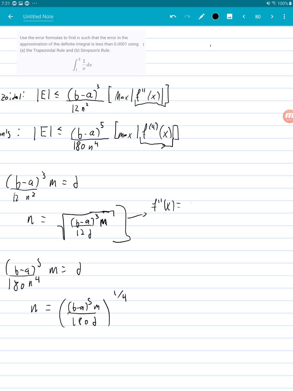
Because Simpson’s Rule is an approximation, there’s always a difference between the calculated value and the true value of the integral. This difference is the error. The error bound formula helps estimate the maximum potential error: |Error| ≤ ((b-a)⁵ / 180n⁴) * M, where ‘M’ is the maximum absolute value of the fourth derivative of f(x) within the interval [a, b].
Minimizing Error
Increasing ‘n’ (the number of subintervals) decreases the error but increases computation time. Adaptive Simpson’s Rule automatically adjusts the subinterval width for optimal precision while minimizing computational effort. However, finding ‘M’ can be challenging and might require advanced mathematical methods or estimations.
Comparing Simpson’s Rule to Other Methods
Simpson’s Rule often outperforms simpler methods like the Trapezoidal Rule, particularly when dealing with curved functions. Ongoing research continues to explore and refine numerical integration techniques, including adaptive methods.
Conclusion
Simpson’s Rule offers a powerful and practical way to estimate areas under curves, facilitating solutions to real-world problems across various disciplines. Online calculators make applying this rule accessible and convenient. While more sophisticated methods exist, understanding the principles of Simpson’s Rule, including error analysis and the choice between the 1/3 and 3/8 rule, empowers you to use the most effective numerical integration technique that suits your specific task. Try exploring our interactive row echelon calculator for further mathematical explorations or delve into the fascinating sinxcosx identity to expand your trigonometric knowledge.
- Senior at What Age: Benefits & Eligibility Guide - March 29, 2025
- Unlocking Senior Benefits: How Old is a Senior? Your Complete Guide - March 29, 2025
- Master Russian Politeness:A Guide to Saying Please - March 29, 2025


![Here are a few title options that incorporate your keywords, reflect current trends, and mirror competitor approaches:Direct & Actionable:AP Calculus BC Score Calculator (2023-2024): Predict & Improve Your Score
Free AP Calculus BC Score Calculator: 2024 Predictions & Exam GuideBenefit-Driven:Get a 5 on the AP Calculus BC Exam: Score Calculator & Study Guide
Ace Your AP Calculus BC Exam: Score Predictor & Prep ResourcesAdding Specificity (if applicable):[Your Website's Name] AP Calculus BC Score Calculator: 2024 ExamTips for Choosing the Best Title:Analyze Competitor Titles: Look at the top-ranking pages for AP Calc BC score calculator. Identify common themes and phrases.
Target Long-Tail Keywords: Consider longer, more specific phrases users might search, like how accurate are AP Calculus BC score calculators.
A/B Testing: If possible, test different titles to see which performs best in terms of clicks and engagement. ap_calc_bc_score_calculator](https://www.lolaapp.com/wp-content/uploads/2024/10/ap_calc_bc_score_calculator-150x150.jpg)


